\section{Introduction}\label{sec1}
Numerical analysis can be seen as the “operational” part of a scientific computation. In particular, a thorough error analysis is necessary for an informed assessment of the quality of any obtained result. Three examples are considered to illustrate different types of errors and error estimation techniques.
Some preliminaries on machine data representation and error analysis are given in Section 2. In Section 3, two methods of evaluating trigonometric functions are compared with respect to precision. Section 4 illustrates the use of iteration for solving the discrete time matrix algebraic Riccati equation. A third example on numerical integration of a stochastic differential equation is given in Section 5, which shows the application of statistical error analysis. Some conclusions are given in Section 6.
\section{Preliminaries}\label{sec2}
A computer handles pieces of information of a fixed size, a \emph{word}. The number of digits in a word is the \emph{word length}. A normalized \emph{floating point representation} of a real number ![]() is a representation in the form
is a representation in the form
![]()
All real numbers ![]() can be expressed in this representation, where the number
can be expressed in this representation, where the number ![]() is the \emph{mantissa},
is the \emph{mantissa}, ![]() is the \emph{base} and
is the \emph{base} and ![]() is the \emph{exponent}. In a computer, the number of digits for
is the \emph{exponent}. In a computer, the number of digits for ![]() and
and ![]() is limited by the word length.
is limited by the word length.
Suppose that ![]() digits are used to represent
digits are used to represent ![]() . Then it is only possible to represent floating point numbers of the form
. Then it is only possible to represent floating point numbers of the form
![]()
where ![]() is the mantissa
is the mantissa ![]() rounded to
rounded to ![]() digits, and the exponent is limited to a finite range
digits, and the exponent is limited to a finite range
![]()
The normalization ![]() ensures that
ensures that ![]() . In the binary system,
. In the binary system, ![]() , so this digit need not be stored. An exception is
, so this digit need not be stored. An exception is ![]() , for which one sets
, for which one sets ![]() , and it is also practical to set
, and it is also practical to set ![]() , the lower limit of the exponent.
, the lower limit of the exponent.
The set of floating point numbers ![]() that can be represented by the system contains exactly
that can be represented by the system contains exactly ![]() numbers. The limited number of digits in the exponent implies that
numbers. The limited number of digits in the exponent implies that ![]() is limited in magnitude to an interval – the \emph{range} of the floating point system. If
is limited in magnitude to an interval – the \emph{range} of the floating point system. If ![]() is larger in magnitude than the largest number in the set
is larger in magnitude than the largest number in the set ![]() , then
, then ![]() cannot be represented at all. The same is true, in principle, of numbers smaller than the smallest nonzero number in the set
cannot be represented at all. The same is true, in principle, of numbers smaller than the smallest nonzero number in the set ![]() .
.
It can be shown that in a floating point system, every real number in the floating point range of ![]() can be represented with a relative error which does not exceed the \emph{machine unit}
can be represented with a relative error which does not exceed the \emph{machine unit} ![]() , which, when rounding is used, is defined by
, which, when rounding is used, is defined by
![]()
In a floating point system, both large and small numbers are represented with the same relative accuracy. For most computers, the machine unit ![]() lies between
lies between ![]() and
and ![]() .
.
The IEEE 754 standard from 1985 for floating point arithmetic is implemented on most chips used for personal computers and workstations. Two main formats, single and double precision, are defined. The standard specifies that arithmetic operations should be performed as if they were first calculated to infinite precision and then rounded off. The default rounding mode is to round to nearest representable number, with round to even in case of a tie. The infinite precision is implemented by using extra guard digits in the intermediate result of the operation before normalization and rounding. In single precision a floating point representation ![]() of a number
of a number ![]() is stored as
is stored as
![]()
where ![]() is the sign (one bit),
is the sign (one bit), ![]() is the exponent (8 bits), and
is the exponent (8 bits), and ![]() is the mantissa (23 bits). If
is the mantissa (23 bits). If ![]() and
and ![]() are two floating point numbers, the corresponding operations are denoted by
are two floating point numbers, the corresponding operations are denoted by
![]()
for the results of floating point addition, subtraction, multiplication and division. These operations have to some degree other properties than the exact arithmetic operations. The associative and distributive laws may fail for addition and multiplication. Consequently, the order of calculation may have a large impact on the error propagation.
An approximation to the machine unit can be determined as ![]() , where
, where ![]() is the smallest floating point number
is the smallest floating point number ![]() such that
such that
![]()
The machine unit ![]() can therefore be regarded as a lower bound for the relative error in any computation, see [1].
can therefore be regarded as a lower bound for the relative error in any computation, see [1].
\subsection{Error Types}
Numerical results are influenced by many types of error. Some sources of error are difficult to influence while others can be reduced or eliminated by changing the computational sequence. Errors are propagated from their sources to quantities computed later, sometimes with a considerable amplification. It is therefore important to distinguish between the new error produced at the computation of a quantity, and errors propagated from the data that the quantity is calculated from. The following types of error are encountered in machine computations.
\subsubsection{Errors in Given Input Data}
Input data can be the results of measurements which have been influenced by errors. A \emph{rounding error} occurs, for example, whenever an irrational number is shortened (“rounded off”) to a fixed number of decimals.
\subsubsection{Errors During the Computations}
The limited word length in a computer or calculator leads at times to a loss of information. There are two typical and important cases:
\begin{itemize}\item If the device cannot handle numbers which have more than, say, ![]() digits, then the exact product of two
digits, then the exact product of two ![]() -digit numbers (which contains
-digit numbers (which contains ![]() or
or ![]() digits) cannot be used in subsequent calculations, but is rounded off. \item When a relatively small term
digits) cannot be used in subsequent calculations, but is rounded off. \item When a relatively small term ![]() is added to
is added to ![]() , then some digits of
, then some digits of ![]() are “shifted out”, and they will not have any effect on future quantities that depend on the value of
are “shifted out”, and they will not have any effect on future quantities that depend on the value of ![]() . The effect of such roundings can be quite noticeable in an extensive calculation, or in an algorithm which is numerically unstable.\end{itemize}
. The effect of such roundings can be quite noticeable in an extensive calculation, or in an algorithm which is numerically unstable.\end{itemize}
\subsubsection{Truncation Errors}
These are errors arising when a limiting process is truncated (broken off) before the limiting value has been reached. Such \emph{truncation error} occurs, for example, when an infinite series is broken off after a finite number of terms, when a nonlinear function is approximated with a linear function, or when a derivative is approximated with a difference quotient (also called \emph{discretization error}).
\subsubsection{Other Types of Errors}
The most important, but sometimes overlooked sources of error are due to simplifications in the mathematical model, and human or machine errors.
Simplifications in the Mathematical Model
In most of the applications of mathematics, one makes idealizations and assumptions in order to formulate a mathematical model. The idealizations and assumptions made may not be appropriate to describe the present problem and can therefore cause errors in the result. The effects of such sources of error are usually more difficult to estimate than errors in given input data, rounding errors during the computations and truncation errors.
Human Errors and Machine Errors
In all numerical work, one must be aware that clerical errors, errors in hand calculation, and misunderstandings may occur. When using computers, one can encounter errors in the program itself, typing errors in entering the data, operator errors, and (more seldom) machine errors.
Errors in given input data and errors due to simplification of the mathematical model are usually considered to be uncontrollable in the numerical treatment. Truncation errors are usually controllable. The rounding error in the individual arithmetic operation is, in a computer, controllable to a limited extent, mainly through the choice of single and double precision. This type of error can also be reduced by reformulation of the calculation sequence.
\subsection{Functions of a Single Variable}
One of the fundamental extensions of a computing device is to have methods to compute \emph{elementary functions}. A function of a single variable is a mapping ![]() where the argument
where the argument ![]() of
of ![]() is a one-dimensional variable. For all calculated quantities, the following definition of absolute and relative error can be applied.
is a one-dimensional variable. For all calculated quantities, the following definition of absolute and relative error can be applied.
Theorem: Let ![]() be an approximate value to an exact quantity
be an approximate value to an exact quantity ![]() . The \emph{absolute error} in
. The \emph{absolute error} in ![]() is
is
![]()
and if ![]() , the \emph{relative error} is
, the \emph{relative error} is
![]()
In many situations one wants to compute error bounds, either strict or approximate, for the absolute or relative error. Since it is sometimes rather hard to obtain an error bound that is both strict and sharp, one often prefers to use less strict but often realistic error estimates, see [1].
To carry out rounding error analysis of an algorithm based on floating point operations, a model of how these operations are carried out is needed. The standard model
![]()
where ![]() is any of the four elementary operations. The model is valid for the IEEE standard.
is any of the four elementary operations. The model is valid for the IEEE standard.
For a function ![]() , elementary results from calculus can be used to give a bound for the error in the evaluated function value. Let
, elementary results from calculus can be used to give a bound for the error in the evaluated function value. Let ![]() be a function of a single variable
be a function of a single variable ![]() and let
and let ![]() . Then
. Then
![]()
where ![]() . Suppose that
. Suppose that ![]() . Then
. Then
![]()
General Error Propagation Formula: Assume that the errors in ![]() are
are ![]() . Then the maximal error in
. Then the maximal error in ![]() has the approximate bound
has the approximate bound
![]()
\subsection{Vectors and Matrices}
A \emph{vector norm} on ![]() is a function
is a function ![]() satisfying
satisfying
\begin{itemize}\item ![]() \item
\item ![]() \item
\item ![]() \end{itemize}
\end{itemize}
The vector norm of a vector ![]() is denoted
is denoted ![]() . The most common vector norms are special cases of the family of \emph{H\”older norms} or \emph{
. The most common vector norms are special cases of the family of \emph{H\”older norms} or \emph{![]() -norms}, defined by
-norms}, defined by
![]()
The ![]() -norm (or \emph{maximum norm}) is defined
-norm (or \emph{maximum norm}) is defined
![]()
An infinite sequence of matrices ![]() is said to converge to
is said to converge to ![]() , that is
, that is ![]() if
if
![]()
From the equivalence of norms in a finite dimensional vector space it follows that the order of convergence is independent of the choice of norm. The particular choice ![]() shows that convergence of vectors in
shows that convergence of vectors in ![]() is equivalent to convergence of the
is equivalent to convergence of the ![]() sequences of scalars formed by the components of the vectors. This conclusion is extended to matrices, see [1].
sequences of scalars formed by the components of the vectors. This conclusion is extended to matrices, see [1].
\subsection{Iteration}
A general idea often used in numerical computation is \emph{iteration}, where a numerical process is applied repeatedly to a problem. As an example, the equation
![]()
can be solved by successive approximation using an initial approximation ![]() . By using the equation
. By using the equation ![]() repeatedly, a sequence of numbers
repeatedly, a sequence of numbers ![]() is obtained that (hopefully) converges to a limiting value
is obtained that (hopefully) converges to a limiting value ![]() , which is a root to the equation. As
, which is a root to the equation. As ![]() grows, the numbers
grows, the numbers ![]() are then successively better and better approximations to the root, that is
are then successively better and better approximations to the root, that is
![]()
so that ![]() satisfies the equation
satisfies the equation ![]() . The iteration is stopped when sufficient accuracy has been attained. Consider a nonlinear equation of the form
. The iteration is stopped when sufficient accuracy has been attained. Consider a nonlinear equation of the form
![]()
Then, for ![]() , the \emph{fixed-point iteration}
, the \emph{fixed-point iteration}
![]()
can be used to find the root to the equation. If ![]() is continuous and
is continuous and ![]() , then
, then ![]() and
and ![]() solves the system
solves the system ![]() .
.
Generally, a vector sequence is said to converge to a limit ![]() if
if
![]()
for some norm ![]() , see [1].
, see [1].
\subsection{Numerical Stochastic Integration}
Consider an initial value problem consisting of an ordinary differential equation and an initial value,
![]()
![]()
There is a multitude of methods available for numerical evaluation of the integral. One simple and common method is the \emph{Euler method}, in which the derivative is approximated with a forward time difference equation as
![]()
for some given time discretization ![]() , which gives the Euler method for the problem
, which gives the Euler method for the problem
![]()
![]()
![]()
For the Euler method, the \emph{local discretization error}, the error introduced in each step of the method, is defined as
![]()
and the \emph{global discretization error}, the total error after ![]() steps, is defined as
steps, is defined as
![]()
A method is \emph{convergent} if the global discretization error converges to zero with the maximum time step ![]() , that is,
, that is,
![]()
where ![]() on any finite time interval
on any finite time interval ![]() . A method is \emph{stable} if the propagated errors remain bounded.
. A method is \emph{stable} if the propagated errors remain bounded.
Now, consider an \emph{It{\^o} process} ![]() satisfying the stochastic differential equation
satisfying the stochastic differential equation
![]()
![]()
For a given discretization ![]() of the time interval
of the time interval ![]() , the \emph{Euler-Maruyama approximation} is the continuous stochastic process
, the \emph{Euler-Maruyama approximation} is the continuous stochastic process ![]() satisfying
satisfying
![]()
for ![]() with initial value
with initial value ![]() ,
, ![]() and
and ![]() . The process is constructed by generating a white noise process approximation
. The process is constructed by generating a white noise process approximation
![]()
of the Wiener process ![]() , that is, the increments of the Wiener process are normally distributed with a variance equal to the time step length. The white noise process therefore has the properties that
, that is, the increments of the Wiener process are normally distributed with a variance equal to the time step length. The white noise process therefore has the properties that
![]()
In order to generate a continuous function, piecewise constant interpolation is performed to give
![]()
with ![]() . Error estimates for deterministic problems cannot be used in this case. However, if the exact solution is known, a statistical analysis based on simulation can be used to determine the global discretization error. By using path-wise approximations, the expectation of the global discretization error is
. Error estimates for deterministic problems cannot be used in this case. However, if the exact solution is known, a statistical analysis based on simulation can be used to determine the global discretization error. By using path-wise approximations, the expectation of the global discretization error is
![]()
The approximation ![]() with maximum step size
with maximum step size ![]() \emph{converges strongly} to
\emph{converges strongly} to ![]() at time
at time ![]() if
if
![]()
The Euler-Maruyama approximation is the simplest useful approximation for stochastic integration. It is, however, not very numerically efficient. A comprehensive discussion on numerical stochastic integration is given in [2].
\section{Evaluation of Trigonometric Functions}\label{sec3}
The evaluation of trigonometric functions consists of two numerical problems; the approximation of the irrational number ![]() – which cannot be expressed in a finite sequence of decimals in a floating point representation – and the evaluation of the trigonometric function using basic operations. A numerical experiment was carried out to compare two different methods of evaluation of a trigonometric function with an exact argument. The machine unit on the computer was determined to be
– which cannot be expressed in a finite sequence of decimals in a floating point representation – and the evaluation of the trigonometric function using basic operations. A numerical experiment was carried out to compare two different methods of evaluation of a trigonometric function with an exact argument. The machine unit on the computer was determined to be ![]() , using the method described in section ??.
, using the method described in section ??.
Hida et al. [3] suggest an algorithm giving a precision of four times that of double precision IEEE arithmetic. The method for computing ![]() and
and ![]() uses argument reduction, look-up tables and Taylor expansions. In order to compute
uses argument reduction, look-up tables and Taylor expansions. In order to compute ![]() , the argument
, the argument ![]() is reduced modulo
is reduced modulo ![]() , so that
, so that ![]() , due to the fact that the sine function is periodic. Noting that sine and cosine functions are symmetric with respect to
, due to the fact that the sine function is periodic. Noting that sine and cosine functions are symmetric with respect to ![]() and
and ![]() , the argument can be reduced modulo
, the argument can be reduced modulo ![]() . In general,
. In general, ![]() can be expressed as
can be expressed as ![]() or
or ![]() , so that it is only necessary to compute
, so that it is only necessary to compute ![]() and
and ![]() with
with ![]() . Finally, let
. Finally, let ![]() , where the integer
, where the integer ![]() is chosen so that
is chosen so that ![]() . With
. With ![]() , the constant
, the constant ![]() .
.
The value of the sine function with an arbitrary argument can be computed by using the relation
![]()
where ![]() is expanded in a Maclaurin series (Taylor expansion around
is expanded in a Maclaurin series (Taylor expansion around ![]() ) and
) and ![]() and
and ![]() are tabulated pre-computed values. These values are computed using the recursive relation
are tabulated pre-computed values. These values are computed using the recursive relation
![]()
![]()
starting with ![]() . By using the trigonometric formulas
. By using the trigonometric formulas
![]()
![]()
all the values for integers ![]() can be computed. Using the reduction of the argument, the convergence rate for the Maclaurin series is significantly increased. The Maclaurin expansion for a function
can be computed. Using the reduction of the argument, the convergence rate for the Maclaurin series is significantly increased. The Maclaurin expansion for a function ![]() is
is
![Rendered by QuickLaTeX.com \[f(x)=\sum_{n=0}^{\infty}\frac{f^{(n)}(0)}{n!}x^n,\quad |x|<\infty,\]](https://www.mathgallery.com/wp-content/ql-cache/quicklatex.com-ecf2e0d21423427d7c0f6e137e598c96_l3.png)
so that
![]()
![]()
![]()
The \emph{remainder} after ![]() terms gives an estimate of the absolute error,
terms gives an estimate of the absolute error,
![]()
for some ![]() . Thus, an upper bound for the absolute error of the trigonometric functions is therefore given by
. Thus, an upper bound for the absolute error of the trigonometric functions is therefore given by ![]() and the number of terms
and the number of terms ![]() can be chosen as to obtain desired accuracy.
can be chosen as to obtain desired accuracy.
Since the tabulated values are determined with the recursive relation above, the function computation are dependent only on the square root operation, apart from the basic operations. The square root is computed using \emph{Netwton’s method} on the function
![]()
which has the root ![]() . This gives the iterative formula
. This gives the iterative formula
![]()
![]()
Newton’s method is quadratically convergent and any degree of accuracy in the result can be obtained with the given precision. The square root is obtained by multiplying the result with ![]() , that is,
, that is, ![]() .
.
If the elementary operations are assumed to be performed without losing precision (according to the IEEE standard), then the calculations of ![]() would benefit from using the above mentioned method due to that the error in the truncated Maclaurin expansion is smaller the closer to zero the argument is.
would benefit from using the above mentioned method due to that the error in the truncated Maclaurin expansion is smaller the closer to zero the argument is.
The computation of ![]() , where the argument is assumed to be exact, was performed on a personal computer, using two methods; the Maclaurin expansion up to 5 terms without argument reduction (method 1, the result denoted
, where the argument is assumed to be exact, was performed on a personal computer, using two methods; the Maclaurin expansion up to 5 terms without argument reduction (method 1, the result denoted ![]() ), and with argument reduction using the above procedure (method 2,
), and with argument reduction using the above procedure (method 2, ![]() ), respectively. The difference in the calculated results between the methods is
), respectively. The difference in the calculated results between the methods is ![]() . The results are summarized in the following table:
. The results are summarized in the following table:

The result by using method 2, ![]() , is here assumed to have the error bound given by the machine unit
, is here assumed to have the error bound given by the machine unit ![]() . The example illustrates how the truncation error depends on the argument. By reducing the argument higher precision can be achieved.
. The example illustrates how the truncation error depends on the argument. By reducing the argument higher precision can be achieved.
If there is an error in the input, the general error propagation formula (see \autoref{sec2}) can be used to estimate the propagated error in the result,
![]()
\section{The Algebraic Riccati Equation}\label{sec4}
Many measurements of events evolving in time can be regarded as signals disturbed by noise representing measurement errors. One mathematical model that can be used to describe this is the \emph{dynamic system}, defined by known \emph{state equations} which has an input signal controlling the states of the system and an output signal, which is the observations of the system states.
A discrete time model can be represented by the matrix equation
![]()
![]()
where ![]() is the discrete time step. In this representation, the vector
is the discrete time step. In this representation, the vector ![]() represents the state of the system, where the number of state variables is equal to the length of
represents the state of the system, where the number of state variables is equal to the length of ![]() .
.
The state at a time ![]() is a linear combination of previous states (at times less or equal to
is a linear combination of previous states (at times less or equal to ![]() ) and a control variable
) and a control variable ![]() with a superimposed white noise process
with a superimposed white noise process ![]() . The linear combinations are given by the matrices
. The linear combinations are given by the matrices ![]() and
and ![]() , respectively. The initial state at time
, respectively. The initial state at time ![]() is
is ![]() . Measurements on the system are represented by the matrix equation
. Measurements on the system are represented by the matrix equation
![]()
where the vector ![]() represents the observed values at time
represents the observed values at time ![]() , that is the measurements of some linear combination of the state variables of the system,
, that is the measurements of some linear combination of the state variables of the system, ![]() at time
at time ![]() , and a noise component,
, and a noise component, ![]() . The linear combinations are defined by the matrices
. The linear combinations are defined by the matrices ![]() and
and ![]() , respectively.
, respectively.
If the input signal is assumed to be constant with an imposed white noise, the \emph{Kalman filter} defines a scheme to obtain the optimal estimation of the actual system states, given the noisy observations ![]() , see for example [4].
, see for example [4].
The Kalman estimator is optimal in the sense that it minimizes the least square error, that is
![]()
The Kalman filter is given by
![]()
![]()
where the Kalman gain ![]() is given by
is given by
![]()
and ![]() is the stationary solution to the discrete matrix \emph{Riccati equation}
is the stationary solution to the discrete matrix \emph{Riccati equation}
![]()
![]()
Normally the \emph{steady-state matrices} ![]() and
and ![]() for
for ![]() are used.
are used.
It can be shown (see [4]), that if the system is \emph{controllable} and \emph{observable}, then the discrete-time algebraic Riccati equation has a unique positive semi-definite solution.
Definition: \emph{Construct the \emph{controllability matrix}
![]()
Then the matrix pair ![]() is called \emph{controllable} if
is called \emph{controllable} if ![]() .}
.}
Definition: \emph{Construct the \emph{observability matrix}
![Rendered by QuickLaTeX.com \[\mathbf{\Omega}=\left(\begin{array}{c} \mathbf{C}\\\mathbf{C}\mathbf{A}\\ \vdots\\\mathbf{C}\mathbf{A}^{n-1}\end{array}\right).\]](https://www.mathgallery.com/wp-content/ql-cache/quicklatex.com-177184106aef12d04c745b98dd273d0b_l3.png)
Then the matrix pair ![]() is called \emph{observable} if
is called \emph{observable} if ![]() .}
.}
As a numerical example, let the vertical motion of a cruising aircraft be modelled by the one-dimensional motion of a particle, that is
![]()
where ![]() is the position of the particle and
is the position of the particle and ![]() is the applied force. If
is the applied force. If ![]() is constant (it is assumed here that
is constant (it is assumed here that ![]() ), then the remaining force can be assumed to be the influence of turbulence on the aircraft motion, which is modelled by the white noise process
), then the remaining force can be assumed to be the influence of turbulence on the aircraft motion, which is modelled by the white noise process ![]() . The tracking system performs measurements of the height
. The tracking system performs measurements of the height ![]() , which are assumed to be disturbed by measurement errors modelled by white noise
, which are assumed to be disturbed by measurement errors modelled by white noise ![]() . Define the state space variables
. Define the state space variables ![]() to be the position and
to be the position and ![]() to be the velocity of the aircraft. Then
to be the velocity of the aircraft. Then
![]()
![]()
so that
![]()
![]()
where the matrices are time-independent and ![]() and
and ![]() are scalar white noise processes. Furthermore, it is assumed that the tracking system is operating in discrete time, sampled with time step
are scalar white noise processes. Furthermore, it is assumed that the tracking system is operating in discrete time, sampled with time step ![]() . If
. If ![]() is small, the applied force can be approximated by a piecewise constant signal. Integration of the state equation gives
is small, the applied force can be approximated by a piecewise constant signal. Integration of the state equation gives
![]()
![]()
by the assumption of the scalar noise process ![]() being constant on
being constant on ![]() and
and ![]() being independent of
being independent of ![]() . Series expansion gives
. Series expansion gives
![]()
and therefore
![]()
![]()
which gives the resulting discrete time state equation
![]()
where ![]() and
and ![]() is the position and velocity of the particle at time
is the position and velocity of the particle at time ![]() , respectively. The system is controllable and observable for
, respectively. The system is controllable and observable for ![]() , since
, since
![]()
The discrete time algebraic Riccati equation can be interpreted as a system of nonlinear equations. The form of the equation suggests that the solution can be found by iterating the Riccati equation.
As initial value, any positive definite matrix, for example ![]() , can be used. The result from each iteration is tested component wise using the maximum norm (see \autoref{sec2}), so that the component wise maximum error is used as a stop condition for the iteration. The result after a few iterations is
, can be used. The result from each iteration is tested component wise using the maximum norm (see \autoref{sec2}), so that the component wise maximum error is used as a stop condition for the iteration. The result after a few iterations is
![]()
with a component wise error of approximately ![]() . The corresponding Kalman gain and filter are, respectively
. The corresponding Kalman gain and filter are, respectively
![]()
![]()
\section{Numerical Solution of a Stochastic Differential Equation}\label{sec5}
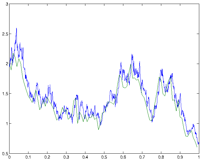
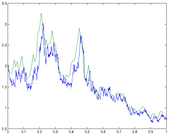
A numerical experiment was performed on the It{\^o} process
![]()
on the interval ![]() . The equation has the exact solution
. The equation has the exact solution
![]()
To make an error estimation on a computer, simulations of the same sample paths of the It{\^o} process and their Euler approximation corresponding to the same sample paths of the Wiener process are repeated ![]() times. The error estimate (see \autoref{sec2}) is given by
times. The error estimate (see \autoref{sec2}) is given by
![Rendered by QuickLaTeX.com \[\hat{\epsilon}=\frac{1}{N}\sum_{k=1}^N|X_{T,k}-Y_{T,k}|.\]](https://www.mathgallery.com/wp-content/ql-cache/quicklatex.com-bb513fbf816dd2e96c9d4d90450938f4_l3.png)
In order to estimate the variance ![]() of
of ![]() , the simulations are arranged into
, the simulations are arranged into ![]() batches of
batches of ![]() simulations each. The average errors
simulations each. The average errors
![Rendered by QuickLaTeX.com \[\hat{\epsilon}_j=\frac{1}{N}\sum_{k=1}^N|X_{T,k,j}-Y_{T,k,j}|\]](https://www.mathgallery.com/wp-content/ql-cache/quicklatex.com-8b92b2d345ca97d58c66eb8385d04420_l3.png)
of the ![]() batches are independent and approximately Gaussian for large
batches are independent and approximately Gaussian for large ![]() . Student’s
. Student’s ![]() -distribution with
-distribution with ![]() degrees of freedom is used to construct a
degrees of freedom is used to construct a ![]() confidence interval
confidence interval ![]() for
for ![]() , where
, where
![Rendered by QuickLaTeX.com \[\hat{\epsilon}=\frac{1}{M}\sum_{j=1}^M\hat{\epsilon}_j=\frac{1}{NM}\sum_{j=1}^M\sum_{k=1}^N|X_{T,k,j}-Y_{T,k,j}|,\]](https://www.mathgallery.com/wp-content/ql-cache/quicklatex.com-0704bc219e963261dba4450f98b78763_l3.png)
![Rendered by QuickLaTeX.com \[\hat{\sigma}_{\epsilon}^2=\frac{1}{M-1}\sum_{j=1}^M(\hat{\epsilon}_j-\hat{\epsilon})^2,\]](https://www.mathgallery.com/wp-content/ql-cache/quicklatex.com-4de0e3e2986e514bafa4417f9b883768_l3.png)
![]()
The Euler method has the order of strong convergence 1/2. The solution was simulated with ![]() steps and the Euler-Maruyama method was used with time step
steps and the Euler-Maruyama method was used with time step ![]() . In order to estimate the global discretization error,
. In order to estimate the global discretization error, ![]() different simulations and approximations were performed
different simulations and approximations were performed ![]() times, which yielded the error estimates
times, which yielded the error estimates
![]()
![]()
An approximate ![]() confidence interval for
confidence interval for ![]() , that is, the expected deviation of the Euler-Maruyama approximation from the exact solution at time
, that is, the expected deviation of the Euler-Maruyama approximation from the exact solution at time ![]() , is therefore given by
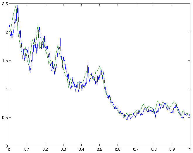
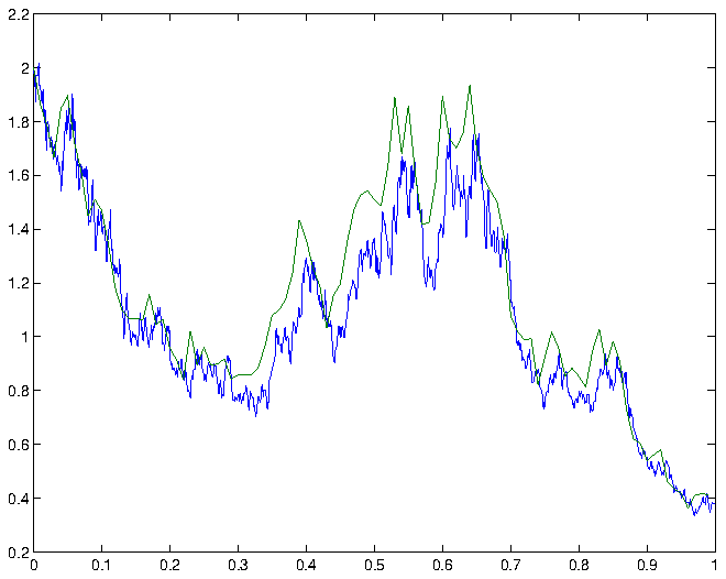
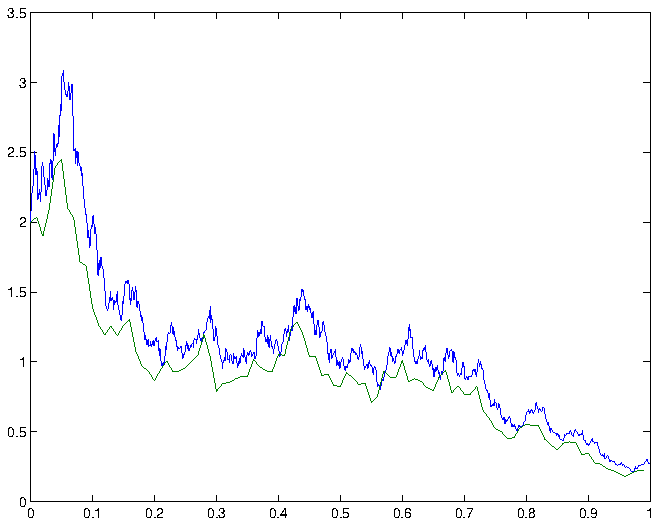
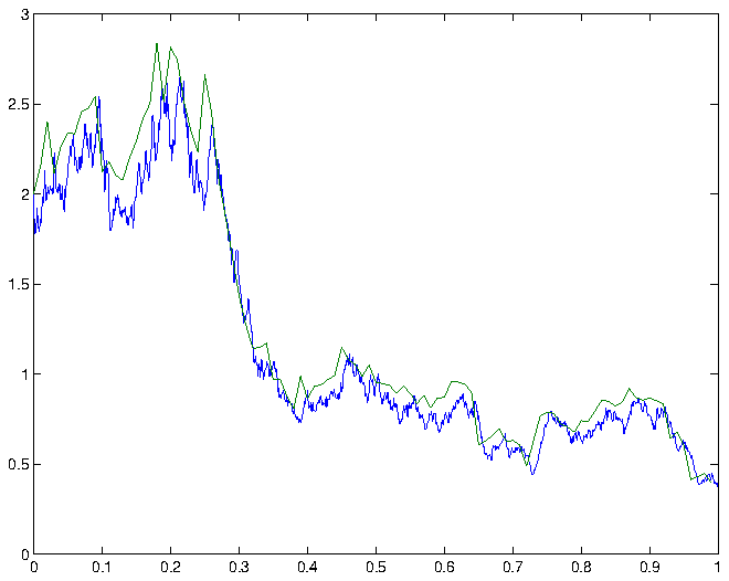
, is therefore given by ![]() . Some simulations and the corresponding Euler-Maruyama approximations are shown in figure 1.
. Some simulations and the corresponding Euler-Maruyama approximations are shown in figure 1.
\section{Conclusion}\label{sec6}
In this paper, three examples are given to illustrate estimation of different types of errors. In numerical computation, it is essential to identify error sources and follow the propagation of errors throughout the calculations. Solving a problem using two different methods is a powerful way to distinguish error sources, when this approach is feasible. Two different methods are used to evaluate a trigonometric function, which reveals the impact of different error sources.
For matrix equations, error estimation is more complex, since a suitable (matrix) norm has to be chosen. The discrete time Riccati equation can be solved by iteration, and the use of the maximum norm as a measure of the error is illustrated in the second example.
For numerical solution methods for stochastic problems, statistical methods have to be used for error estimation. This approach is illustrated in the example of numerical solution of a stochastic differential equation.
\section{References}
[bibshow][bibcite key=Approx,SDE,Hida,Control][/bibshow]
